728x90

텐서에 익숙해져있다가 파이토치로 넘어가려니 아직은 어렵다...
+이번 책 끝내고, 나중에 여유 좀 생기면 파이토치 튜토리얼도 봐야지!
PyTorch 소개
Introduction|| Tensors|| Autograd|| Building Models|| TensorBoard Support|| Training Models|| Model Understanding 아래 영상이나 youtube 를 참고하세요. PyTorch Tensors: 03:50 에 시작하는 영상을 시청하세요. PyTorch를 import할 것
tutorials.pytorch.kr
#1. 파이토치 기초
파이토치 아키텍처
파이토치 API
- torch : GPU 지원 텐서 패키지
- torh.autograd : 자동 미분 패키지. 신경망에 변경이 생길 경우 즉시 계산할 수 있음
- torch.nn : 신경망 구축
- torch.multiprocessing : 서로 다른 프로세스에서 동일한 데이터(텐서)에 접근, 사용할수 있게 함
- torch.utils : torch.utils.data.DataLoader 를 통해 모델에 데이터 제공, torch.utils.checkpoint 통한 모델 검사 등 수행
이 외 파이토치 엔진, 연산처리 등이 또한 있음
파이토치 기초 문법
1. 텐서 생성 및 변환
import torch

#텐서 생성
torch.tensor([[1,2],[3,4]], device = "cuda:0") #GPU에 텐서 생성
torch.tensor([[1,2],[3,4]], dtype = torch.float64) #유형 지정

#텐서 배열로 변경
temp = torch.tensor([[1,2],[3,4]])
temp.numpy()

temp2 = torch.tensor([[1,2],[3,4]], device = "cuda:0")
temp.to("cpu").numpy()
2. 텐서 인덱스 조작
배열과 동일하게 인덱스, 슬라이싱 가능
3. 텐서 연산 및 차원 조작
텐서 연산
- 유의사항 : 텐서 간 타입이 다르면 연산이 불가능 (e.g. FloatTensor(32bit) - DoubleTensor(64bit) 불가능)
v = torch.tensor([1,2,3])
w = torch.tensor([3,4,6])

w-v
#tensor([2,2,3])
텐서 차원 조작
temp = torch.tensor([[1,2],[3,4]])

temp.view(4,1)    #4*1로 변환
temp.view(-1)     #1차원 벡터로 변환
temp.view(1,-1)   # (1,-1) = (1,?) 다른 차원으로 부터 해당 값을 유추.
temp.view(-1,1)
데이터 준비
1. 파일을 불러와서 사용하는 경우
import pandas as pd
import torch

data = pd.read_csv("파일경로")

#csv 파일의 컬럼을 넘파이 배열로 받아 tensor로 바꿔주는 것
x = torch.from_numpy(data['불러오려는 열 이름'].values).unsqueez(dim=1).folat()
2. 커스텀 데이터셋을 만들어서 사용하는 경우
데이터를 한번에 메모리에 불러오면 비효율적이므로 데이터를 조금씩 나눠서 불러오는 방식
import pandas as pd
import torch
from torch.utils.data import Dataset
from torch.utils.data import DataLoader

#클래스 정의

class CustomDataset(torch.utils.data.Dataset):
	def__init__(self,csv_file):          #필요한 변수 선언, 데이터 셋 전처리
    	self.label = pd.read_csv

    def__len__(self):           # 데이터셋 총 샘플 수
    	return len(self.label)

    def__getitem__(self.index): #특정 데이터를 가져오는 함수 (인덱스번째 데이터 반환)
    	sample = torch.tensor(self.label.iloc[index, 0:3]).int()
        label = torch.tensor(self.label.iloc[index,3]).int()
        return sample, label

#적용

tensor_dataset = CustomDataset('파일경로')
dataset = DataLoader(tensor_dataset, batch_size=4, shuffle=True)
3. 파이토치 자체 데이터 사용하는 경우
#터미널에 리퀘스트 설치
pip install requests

#여기부터 불러오는법

import torchvision.transforms as transforms

mnist_transform = transforms.Compose([
	transforms.ToTensor(),
    transforms.Normalize((0.5,),(1.0,))

from torchvision.datasets import MNIST
import requests

dowonload_root = '다운받을 경로'
train_dataset = MNIST(download_root, transform=mnist_transform, train=True,download=True)
모델 정의
1. 단순 신경망 정의
nn.Module() 상속 받지 않는 단순한 모델 생성 시 사용
model = nn.Linear(in_features=1, out_features=1, bias=True)2. nn.Module() 상속하여 정의
class MLP(Module):
	#모델에서 사용할 모듈 (Linear,Conv2D..)과 활성화 함수 정의
	def __init__ (self,inputs):
    	super(MLP, self).__init__()    #부모 클래스인 Module에 접근
        self.layers = Linear(inputs,1) #계층 정의
        self.activation = Sigmoid()
    #모델에서 실행되어야 하는 연산을 정의
    def forward(self,X):
    	X = self.layer(X)
        X = self.activation(X)
        return X
3. Sequential 신경망 정의
__init__에서 사용할 네트워크 모델 정의해주고 forward 함수에서 모델에서 실행되어야 할 계산을 가독성 높게 작성해줌
import torch.nn as nn

class MLP(nn.Module):
	def __init__(self):
    	super(MLP,self).__init__()
        self.layer1 = nn.Sequential(
        	nn.Conv2D(in_channels=3, out_channels=64, kernel_size=5),
            nn.Relu(inplace=True),
            nn.MaxPool2d(2))

        self.layer2 = nn.Sequential(
        	nn.Conv2D(in_channels=64, out_channels=30, kernel_size=5),
            nn.Relu(inplace=True),
            nn.MaxPool2d(2))

        self.layer3 = nn.Sequential(
        	nn.Linear(in_features=30*5*5, out_features=10, bias=True),
            nn.Relu(inplace=True),)

    def forward(self,x):
    	x = self.layer1(x)
        x = self.layer2(x)
        x = x.view(x.shape[0],-1)
        x = self.layer3(x)
        return x
4. 함수로 신경망 정의
변수에 저장한 계층들을 재사용할 수 있으나 모델이 복잡해질 수 있음
def MLP(in_features = 1, hidden_featrues = 20, out_features=1):
	hidden = nn.Linear(in_features = in_features, out_features = hidden_features, bias = True)
    activation = nn.ReLU()
    output = nn.Linear(in_features = hidden_features, out_features=out_features, bias= True)
    net = nn.Sequential(hidden,activation,output)
    return net
모델의 파라미터 정의
- 손실함수
- BCELoss : 이진분류 시 사용
- CrossEntropy : 다중 클래스 분류 시 사용
- MSELoss : 회귀 시 사용
- 옵티마이저
- step() 메서드를 통해 파라미터를 전달받게됨. 모델 파라미터 별로 다른 기준을 적용시킬 수 있음
- torch.optim.Optimizer(params,defaults) 옵티마이저 기본 클래스
- zero_grad() 메서드는 옵티마이저에 사용된 파라미터들의 기울기를 0 으로 만듬
- torch.optim.lr_scheduler : 에포크에 따라 학습률 조정 가능
- optim.Adam, optim.SparseAdma, optim.Adamax, optim.Adagrad, optim.ASGD, optim.LBFGS, optim.SGD ..
- 학습률 스케쥴러 : 미리 지정한 횟수의 에포크를 지날 때 마다 학습률을 감소시켜서 학습 초기에는 빠른 학습을 진행하다 전역 최소점(global minima) 근처에서 학습률을 줄여서 최적점을 찾아갈 수 있게 함
- optim.lr_scheduler.LambdaLR : lambda 이용하여 그 함수 결과를 학습률로 설정
- optim.lr_scheduler.StepLR : 특정 step 마다 학습률을 감마 비율만큼 감소
- optim.lr_scheduler.MultiStepLR : 특정 단계가 아닌 지정된 에포크 마다 학습률을 감마 비율로 감소
- optim.lr_scheduler.ExponentialLR : 에포크 마다 이전 학습률에 감마 만큼 곱함
- optim.lr_scheduler.CosineAnnealingLR : 학습률을 코사인 함수 형태처럼 변화시킴 와리가리
- optim.lr_shceduler.ReduceLROnPlateau : 학습이 잘 되고 있는지 여부에 따라 동적으로 학습률 변화시킴
- 지표 : 훈련과 테스트 단계 모니터링
모델 훈련
- 모델 학습 과정
- 모델, 손실 함수, 옵티마이저 정의
- optimizer.zero_grad()로 기울기 초기화
- 순환신경망(RNN)에서는 새로운 기울기 값을 이전 기울기값에 누적하여 계산하기 때문에 이를 사용할 필요 없음
- ouput = model(input) : 출력 계산하며 전방향 학습
- loss = loss_fn(output,target) : 오차 계산
- loss.backward() : 역전파 학습. 기울기 자동 계산. 이 때 배치가 반복될때마다 오차가 중첩적으로 쌓이므로 매번 기울기 초기화
- optimizer.step() : 기울기 업데이트
for epoch in range(100):

	yhat = model(x_train) #출력값
    loss = criterion(yhat, y_train) #yhat:output, y_train:target
    optimizer.zero_grad()
    loss.backward()
    optimizer.step()
모델 평가
#터미널에 평가 위해 설치

pip install torchmetrics

#1. 함수 사용하여 평가하는 경우

import torch
import torchmetrics

preds = torch.radn(10,5).softmax(dim=1)
target = torch.randint(5,(10,))
acc = torchmetrics.functional.accuracy(preds,target)

#2. 모듈 사용하여 평가하는 경우

import torch
import torchmetrics
metric = torchmetrics.Accuracy() #초기화

n_batches = 10
for i in range(n_batches):
	preds = torch.randn(10,5).softmax(dim=1)
    target = torch.randint(5,(10,))

    acc = metric(preds,target)
    print(f"accuracy on batch {i} : {acc}")    #현재 배치에서의 모델 평가 정확도

acc= metric.compute()
 print(f"accuracy on all data: {acc}")  # 전체 모델 평가 정확도
실습
1. 데이터 전처리
import torch
import torch.nn as nn
import numpy as np
import pandas as pd
import matplotlib.pyplot as plt
import seaborn as sns
%matplotlib inline

dataset = pd.read_csv('~/chap02/data/car_evaluation.csv')

categorical_columns = ['price', 'maint', 'doors', 'persons', 'lug_capacity', 'safety']

#1. 카테고리 컬럼을 astype을 통해 범주형으로 변환
for category in categorical_columns :
    dataset[category] = dataset[category].astype('category')

#2. 범주형 데이터(단어)를 숫자(넘파이 배열)로 변환하기 위해 cat.codes 사용
price = dataset['price'].cat.codes.values
maint = dataset['maint'].cat.codes.values
doors = dataset['doors'].cat.codes.values
persons = dataset['persons'].cat.codes.values
lug_capacity = dataset['lug_capacity'].cat.codes.values
safety = dataset['safety'].cat.codes.values

#3. 넘파이 객체들을 합치기 위해 np.stack 사용 (np.stack 은 새로운 차원을 생성해주며 합치는 배열간 차원 즉 Shape가 같아야 함)
categorical_data = np.stack([price,maint,doors,persons,lug_capacity,safety],1)
# 확인을 원한다면 이 코드로 확인 categorical_data[:10]

#4. 넘파이 배열을 텐서로 변환
categorical_data = torch.tensor(categorical_data, dtype = torch.int64)

#5. label 텐서로 변환
outputs = pd.get_dummies(dataset.output)
outputs = outputs.values
outputs = torch.tensor(outputs).flatten()  #1차원으로 변환

#6. 범주형 칼럼을 N차원으로 변환
###이미 앞에서 범주형 데이터들 배열로 만들어줬는데, 단어 간의 세부 관계?를 잘 파악하기 위해서 기존 데이터셋에서 워드임베딩을 한다고함...
###일단 그래서 넘파이 배열 만든 걸 차원으로 변환...보통 칼럼의 고유값수, 차원의수(고유값수 절반)이 대세인가봄..
categorical_columns_sizes = [len(dataset[column].cat.categories) for column in categorical_columns]
categorical_embedding_sizes = [(col_size,min(50,(col_size+1)//2)) for col_size in categorical_columns_sizes]

#7. 데이터셋 분리

total_records = 1728
test_records = int(total_records*.2)

categorical_train_data = categorical_data[:total_records-test_records]      #0~80%
categorical_test_data = categorical_data[total_records-test_records:total_records]  #80~100
train_outputs = outputs[:total_records-test_records]
test_outputs = outputs[total_records-test_records:total_records]
2. 모델 네트워크 생성
class Model(nn.Module):
    def __init__(self,embedding_size,output_size,layers,p=0.4):     #p=dropout
        super().__init__() #부모클래스인 self에 접근
        self.all_embeddings = nn.ModuleList([nn.Embedding(ni,nf) for ni,nf in embedding_size])
        self.embedding_dropout = nn.Dropout(p)

        all_layers=[]
        num_categorical_cols = sum((nf for ni,nf in embedding_size))
        input_size = num_categorical_cols

        for i in layers:
            all_layers.append(nn.Linear(input_size,i))
            all_layers.append(nn.ReLU(inplace=True))
            all_layers.append(nn.BatchNorm1d(i))      #배치정규화
            all_layers.append(nn.Dropout(p))
            input_size = i

        all_layers.append(nn.Linear(layers[-1], output_size))
        self.layers = nn.Sequential(*all_layers)

    def forward(self,x_categorical):
        embeddings = []
        for i,e in enumerate(self.all_embeddings):
            embeddings.append(e(x_categorical[:,i]))

        x = torch.cat(embeddings,1)
        x = self.embedding_dropout(x)
        x = self.layers(x)

        return x
3. 모델 훈련
model = Model(categorical_embedding_sizes,4,[200,100,50],p=0.4) #임베딩 크기, 출력값크기, 은닉층 뉴런, 드롭아웃
print(model)
Model(
(all_embeddings): ModuleList(
(0): Embedding(4, 2)
(1): Embedding(4, 2)
(2): Embedding(4, 2)
(3): Embedding(3, 2)
(4): Embedding(3, 2)
(5): Embedding(3, 2)
)
(embedding_dropout): Dropout(p=0.4, inplace=False)
(layers): Sequential(
(0): Linear(in_features=12, out_features=200, bias=True)
(1): ReLU(inplace=True)
(2): BatchNorm1d(200, eps=1e-05, momentum=0.1, affine=True, track_running_stats=True)
(3): Dropout(p=0.4, inplace=False)
(4): Linear(in_features=200, out_features=100, bias=True)
(5): ReLU(inplace=True)
(6): BatchNorm1d(100, eps=1e-05, momentum=0.1, affine=True, track_running_stats=True)
(7): Dropout(p=0.4, inplace=False)
(8): Linear(in_features=100, out_features=50, bias=True)
(9): ReLU(inplace=True)
(10): BatchNorm1d(50, eps=1e-05, momentum=0.1, affine=True, track_running_stats=True)
(11): Dropout(p=0.4, inplace=False)
(12): Linear(in_features=50, out_features=4, bias=True)
)
)
4. 파라미터 정의
#손실함수, 옵티마이저
loss_function = nn.CrossEntropyLoss()
optimizer = torch.optim.Adam(model.parameters(),lr=0.001)

#GPU사용 여부
if torch.cuda.is_available():
    device = torch.device('cuda')
else:
    device = torch.device('cpu')
5. 모델 학습
epochs = 500

aggregated_losses=[]
train_outputs = train_outputs.to(device=device, dtype=torch.int64)

for i in range(epochs):
    i+=1
    y_pred = model(categorical_train_data).to(device)
    single_loss = loss_function(y_pred,train_outputs)
    aggregated_losses.append(single_loss)

    if i%25==1:
        print(f'epoch:{i:3} loss:{single_loss.item():10.8f}')

    optimizer.zero_grad()
    single_loss.backward()
    optimizer.step()
5. 테스트 데이터셋으로 모델 예측 : 오차
test_outputs = test_outputs.to(device=device, dtype=torch.int64)
with torch.no_grad():
    y_val = model(categorical_test_data)
    loss = loss_function(y_val,test_outputs)
print(f'Loss:{loss:.8f}')
#Loss:0.55113798
6. 모델 예측값 확인
#가장 큰 값을 갖는 인덱스 확인
###인덱스가 0인 값이 인덱스가 1인 값보다 크기 때문에 처리된 출력??이???0이다???
y_val = np.argmax(y_val,axis=1)
print(y_val[:5])

#정확도, 정밀도, 재현율 확인
from sklearn.metrics import classification_report, confusion_matrix, accuracy_score
print(confusion_matrix(test_outputs,y_val))
print(classification_report(test_outputs,y_val))
print(accuracy_score(test_outputs, y_val))
[[259 0]
[ 85 1]]
precision recall f1-score support
0 0.75 1.00 0.86 259
1 1.00 0.01 0.02 86
accuracy 0.75 345
macro avg 0.88 0.51 0.44 345
weighted avg 0.81 0.75 0.65 345
0.7536231884057971딥러닝 분류 모델의 성능 평가 지표
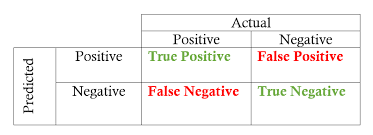
- 정확도(Accuracy) : 전체 예측 건수에서 정답을 맞춘 건수의 비율
- (True Positive + True Negative) / (모든 경우의 수)
- 재현율(Recall) : 실제 정답이 1일때, 모델이 1로 예측한 비율 (처음부터 데이터가 1일 확률이 적을 때 사용)
- True Positive / True Positive + False Negative
- 정밀도(Precision) : 모델이 1로 예측한 것 중에 실제로 정답이 1인 비율
- True Positive / True Positive + False Positive
- F1 Score : 정밀도-재현율의 트레이드 오프 문제를 해결하기 위해 조화 평균을 구한 것
- 2 * (Precision * Recall ) / (Precision + Recall)
'👩💻LEARN : ML&Data > Book Study' 카테고리의 다른 글
| [알고리즘 구현으로 배우는 선형대수] #6. 역행렬 (0) | 2023.04.10 |
|---|---|
| [알고리즘 구현으로 배우는 선형대수] #5. 행렬식 (0) | 2023.04.10 |
| [알고리즘 구현으로 배우는 선형대수] #4. 선형 시스템 (0) | 2023.04.08 |
| [알고리즘 구현으로 배우는 선형대수] #3. 다양한 행렬 (0) | 2023.04.07 |
| [알고리즘 구현으로 배우는 선형대수] #2. 행렬 (5) | 2023.03.17 |